flowchart TD
  A[Data] -->|Check Variance| B{F-test}
  B -->|F-test p > 0.05| C[Student's t-test]
  B -->|F-test p <= 0.05| D[Welch's t-test]
About me
- Rodolfo Lourenzutti
- BSc and MSc in Statistics and PhD in Computer Science (all in Brazil);
- Postdoctoral Researcher at the University of Alberta (Dept. of Civil Engineering);
- Postdoctoral Fellow of Teaching and Learning at UBC (Dept. of Computer Science and Master of Data Science Program);
- Currently an Associate Professor of Teaching at the Statistics Department at UBC;
Teaching
- I have two main values that guide my teaching philosophy:
- Motivation
- Active learning
- Nominated an Open Education Resource Champion at UBC;
- Nominated for Killam Teaching Award at UBC (results still pending);
About this seminar
I believe the topic of “data-driven analysis” to be highly relevant for our students, but also often overlooked;
I have been spending some energy trying to figure out how (and what) to teach this topic in a way that is relatable and informative for students.
Logistics
- My focus is undergraduate students – past inference courses;
- Maybe a modelling course – SDS 334?
- Or a case study in data science – SDS 357?
- There will be some activities that might be weird for this audience (e.g., think-pair-share).
- How to handle this?
- Students told me I’m a bit loud. I also like to provoke engagement.
- Again, it might be a bit weird, but bear with me :)
Pitfalls of Adaptive Data Analysis
How sequential decisions can invalidate your inference
Learning Goals
By the end of this lecture, you will be able to:
Recognize how “data-driven” decisions (like pre-testing assumptions or selecting variables based on data) can invalidate standard p-values.
Demonstrate through simulation how “Post-Selection Inference” inflates Type I error rates.
Implement data splitting as a practical solution to ensure valid inference.
Adaptive data analysis is everywhere
- Data scientists often make decisions based on data analysis results, such as:
- Handling outliers
- Deciding which statistical tests to use
- Selecting models
- Choosing which features to include in a model
- When your choice of model is driven by the data, the model itself becomes a random variable.
Data-Driven decisions: the impact on inference
This “methodological randomness” is not accounted for by standard inferential methods, but it is often overlooked.
Unfortunately, this can lead to “invalid” inference by inflating error rates.
- Today we will begin exploring this issue.
Part I: Pre-testing
Do it or not do it? That is the question.
Scenario: The Bottling Plant
Suppose we want to evaluate two different bottling machines (A and B). We need to ensure they fill bottles to the same average volume (\(\mu_A = \mu_B\)).
We collect a sample of filled bottles from each machine:
- Machine A: \(\bar{x}_A = 503.2\) ml
- Machine B: \(\bar{x}_B = 499.5\) ml
- Question: Can we conclude that the machines have different mean fill volumes?
- Noooooooo!! These are observed statistics, this difference could be due to chance.
Which test should we use?
- We need to test \(H_0: \mu_A = \mu_B\) vs \(H_A: \mu_A \neq \mu_B\).
- Student’s \(t\)-test: Assumes equal variances (\(\sigma_A = \sigma_B\)).
- Welch’s \(t\)-test: Robust to unequal variances.
- Think pair-share activity:
If the variances are equal, which test should we use? More importantly, why is that? What is the advantage of the chosen test?
Why is it “dangerous” to use \(t\)-test if the variances are unequal?
How would you decide which test to use? Would you check the variances first? If so, how?
Are the variances equal?
- A common instinct is to check the data first, and then decide which test to use based on what we find. For example:
- Look at the data:
- Check if the sample variances look similar.
- Or even run an \(F\)-test or Levene’s test to check whether group variances are equal.
- If we fail to reject the null hypothesis: Yay! We can use the standard Student’s \(t\)-test.
- If we reject the null hypothesis: We use Welch’s \(t\)-test as a fallback.
- This image illustrates the concept of “data-driven decisions” — letting the data choose our inferential method.

iClicker 1
Suppose that both machines have the exact same average fill volume. We want to test \(H_0: \mu_A = \mu_B\) vs \(H_A: \mu_A \neq \mu_B\).
Which hypothesis is true?
- \(H_0\).
- \(H_A\).
- It will depend on the value of the test statistic.
- Not enough information to answer this question (e.g., at what significance level?).
iClicker 1: Solution
Suppose that both machines have the exact same average fill volume. We want to test \(H_0: \mu_A = \mu_B\) vs \(H_A: \mu_A \neq \mu_B\).
Which hypothesis is true?
- \(H_0\leftarrow\) Correct!
- \(H_A\)
- It will depend on the value of the test statistic.
- A hypothesis is either true or false, regardless of the data. The data are affected by the true state of the world, but they do not determine it.
- Not enough information to answer this question (e.g., at what significance level?).
- The significance level is a threshold for making a decision based on the data, but it does not affect the truth of the hypotheses.
A common source of confusion
Important: the truth vs the decision
It is important to distinguish between the underlying true state (the true hypothesis) and the decision you make based on the data.
iClicker 2
Suppose that both machines have the exact same average fill volume. We want to test \(H_0: \mu_A = \mu_B\) vs \(H_A: \mu_A \neq \mu_B\) at \(\alpha = 0.05\) significance level.
- If we use a valid test and conduct this test 10,000 times, how many times do you expect to reject \(H_0\)?
- Approximately 500 times.
- Approximately 9500 times.
- It depends on the sample size.
- Who knows? Everything is random!
iClicker 2: Solution
Suppose that both machines have the exact same average fill volume. We want to test \(H_0: \mu_A = \mu_B\) vs \(H_A: \mu_A \neq \mu_B\) at \(\alpha = 0.05\) significance level.
- If we use a valid test and conduct this test 10,000 times, how many times do you expect to reject \(H_0\)?
- Approximately 500 times.\(\leftarrow\) Correct!
- \(\alpha\) is the probability of rejecting a true null hypothesis. Valid tests must control this at the nominal level (0.05 in this case).
- Approximately 9500 times.
- It depends on the sample size.
- Who knows? Everything is random!
- Approximately 500 times.\(\leftarrow\) Correct!
A simulation study: Parameter setup
- Imagine the truth is that both machines have the exact same average fill volume (\(H_0\) is true), but the older Machine A has slightly higher variability in the volumes it outputs.
- \(\mu_A = \mu_B = 500\) ml;
- Note: In practice, we would never know the true means.
- \(\sigma_A = 3\) ml and \(\sigma_B = 2.5\) ml.
- Also usually unknown in practice.
- We will take 10,000 samples of size 20 from Machine A and size 100 from Machine B (both normally distributed).
A simulation study: the code
Exercise 1: Type I Error rates
Exercise 1: Using the data frame results, calculate the proportion of times we rejected \(H_0\) (i.e., p-value < 0.05) for each of the three testing approaches: (1) Student’s \(t\)-test, (2) Welch’s \(t\)-test, and (3) the “Data-Driven” conditional approach.
Exercise 2
Exercise 2: Compute the Type I Error of the “Data-Driven” approach stratified by the F-test decision. Calculate the rejection rate when: (a) the F-test failed to reject (\(p > 0.05\)) and (b) when the F-test rejected (\(p \leq 0.05\)).
Why? We want to see which branch of our decision tree is causing the inflated overall error rate.
Conclusions
- Even though the t-test was used only when the variances appeared “similar,” it still had an inflated Type I error rate.
- Failing to reject the equality of the variance does not guarantee that the variances are actually equal.
- This misalignment between the true variance structure and our chosen test affects the Type I error (positively or negatively, depending on the scenario).
- Failing to reject the equality of the variance does not guarantee that the variances are actually equal.
- Welch’s test had a valid Type I error rate, but using it only when the F-test rejected produced an error rate much smaller than 0.05.
- This is the other side of the coin: Even the Welch test that is applicable in either scenario is being affected by this conditional use.
Remedy: default to Welch’s t-test
While different values of the parameters (sample sizes, variances, etc.) can lead to different error rates, the main point stands: running an F-test before a t-test is not good practice.
The solution here is simple: just default to Welch’s t-test, which is robust to unequal variances, and the power loss is minimal when the variances are actually equal.
Questions?
Post-Selection Inference
A harder problem
Model Selection
- There are many aspects involved in selecting a model that go beyond variable selection:
- Do we want to assume a functional form for the relationship between \(Y\) and \(\mathbf{X}\) (e.g., linear, quadratic, exponential, logarithmic)?
- Prediction performance.
- Is model interpretability important?
- Today we will focus on selecting multiple linear regression models, which comes down to variable selection.
Model Comparison and Selection
We have learned many ways to compare models: (1) \(C_p\), (2) AIC, (3) BIC, (4) F-test, and (5) cross-validation MSE.
and different techniques to search for a good model:
- Stepwise algorithms (e.g., forward selection, backward selection)
- LASSO
- All of these methods are “data-driven” in the sense that they use the data to select the model.
- In other words, the model is data-dependent, and it is not fixed before we see the data.
The problem
- You have learned how to make inferences (e.g., compute confidence intervals and perform hypothesis tests) for a fixed linear model.
- Do these model selection algorithms affect the inference about the parameters of the model?
- To answer these questions, we will again resort to a simulation study!
The problem with double dipping
The problem with using the same data for model selection and inference is that we become overconfident.
The sampling distribution is not what we assume it is, which leads to:
- artificially lower p-values (leads to inflated Type I error);
- artificially narrower confidence intervals;
Simulation Scenario
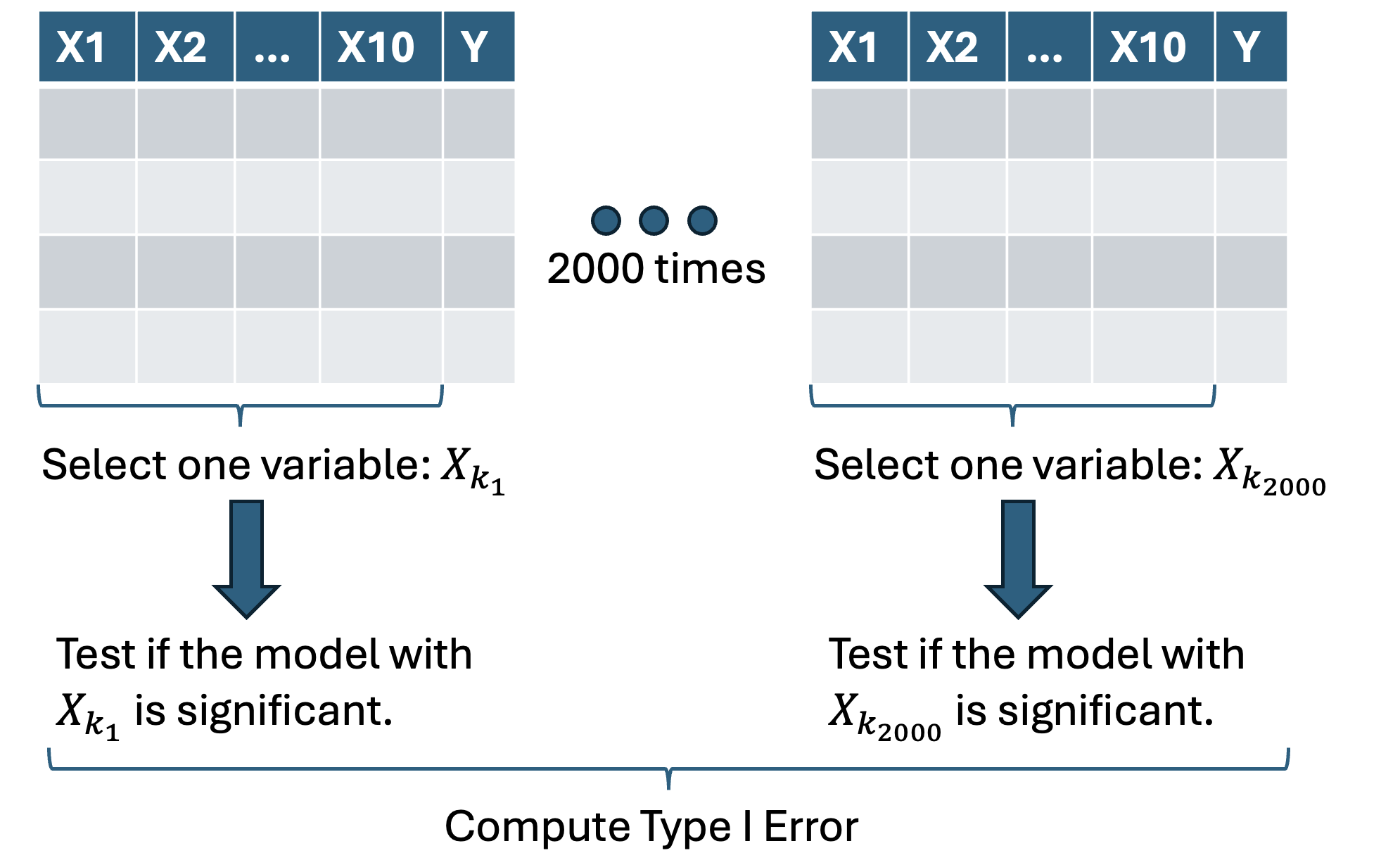
- We will consider a response variable \(Y\) and \(p=10\) covariates. However, none of the covariates affect \(Y\); they are all independent (we already know the truth).
Generate 100 observations of each variable from a normal distribution.
Apply only the first step of forward selection. In other words, we will add only one variable among ten potential candidates.
- The metric we are going to use is the F statistic.
Finally, we will test whether the selected covariate is significant at the 5% level.
replicatethis study 2,000 times and compute how many times we reject \(H_0\).
Diagram of the simulation
iClicker 3
What is the correct decision for our hypothesis?
A. Reject \(H_0\).
B. Do not reject \(H_0\).
C. Depends on the data.
iClicker 3: Solution
What is the correct decision for our hypothesis?
A. Reject \(H_0\).
B. Do not reject \(H_0\). \(\leftarrow\) Correct!
C. Depends on the data.
iClicker 4
This simulation will help us estimate the …
A. Power of the test.
B. Type I Error Rate.
C. Probability of making an error.
D. None of the above.
iClicker 4: Solution
This simulation will help us estimate the …
A. Power of the test.
B. Type I Error Rate. \(\leftarrow\) Correct!
C. Probability of making an error.
D. None of the above.
iClicker 5
What should be the probability of rejecting \(H_0\)?
A. \(5\%\).
B. \(95\%\).
C. Depends on the true value of \(\beta\), which is unknown.
D. None of the above.
iClicker 5: Solution
What should be the probability of rejecting \(H_0\)?
A. \(5\%\). \(\leftarrow\) Correct!
B. \(95\%\).
C. Depends on the true value of \(\beta\), which is unknown.
D. None of the above.
The simulation
- Here are the results:
- At this point, I don’t want you to worry about the code.
[1] "Out of the 2000 simulations, we rejected H0 763 times."[1] "Type I Error Rate: 0.3815"- This is almost 8 times the nominal significance rate of 5%.
Why did this happen?
- We selected the variable with the highest F-statistic from 10 candidates.
- In the noise-only world, we optimized the noise;
- That variable’s F-statistic is naturally inflated because we cherry-picked it.
- When we then test that same variable using the same data, we are testing an inflated effect size.
- The p-value reflects a different (larger) signal than what we’d see in a new sample.
Is \(H_0\) really false?
In this case, we knew that \(H_0\) was true. But in practice, we do not know.
So how can we trust that we are rejecting \(H_0\) because the variable is truly important rather than because our Type I error probability is inflated?
- What to do?
- This is a hard problem and an active area of research in statistics and machine learning.
Data Splitting
- A possible solution for this is to split your data into two independent sets:
- A “search split” (e.g., 50% of data): use to select variables.
- An “inference split” (e.g., 50% of data): use to perform inference (p-values, CIs).
Intuition: if a variable is truly important, it will be important in both splits.
Trade-off: We sacrifice a large chunk of our data for search, which increases the standard error in the inference step:
- Wider confidence intervals
- Less powerful hypothesis tests
- But: inference is now valid at the stated significance level.
Summary
Data-driven decisions can lead to invalid inference by affecting Type I error rates.
In the case of pre-testing for variances, we can just default to Welch’s t-test, which is robust to unequal variances.
In the case of model selection, data splitting is a practical approach to mitigate the issue, but it comes with trade-offs:
- reduces power;
- widens confidence intervals;
- but gives you valid inference.
Q&A
Thank you!
Questions?
© 2026 Rodolfo Lourenzutti CC-BY-SA-NC 4.0