Module 6: Simulation-based hypothesis testing

Learning objectives

Give an example of a question you could answer with a hypothesis test.
Differentiate composite vs. simple hypotheses.
Given an inferential question, formulate null and alternative hypotheses to be used in a hypothesis test.
Identify the steps and components of a basic hypothesis test (“there is only one hypothesis test”).
Write computer scripts to perform hypothesis testing via simulation, randomization and bootstrapping approaches, as well as interpret the output.
Describe the relationship between confidence intervals and hypothesis testing.
Discuss the potential limitations of this simulation approach to hypothesis testing.

Today’s goal

Our goal:
1. understand hypothesis testing framework;
2. test hypothesis through simulation;

Inferential goals: Estimation vs Hypothesis Testing

Estimation vs Hypothesis Testing

In estimation we are interested in estimating a parameter of interest.
- Usually answering questions like “how much”, “how many”, “what is the value of” etc.
In hypothesis testing we are interested in testing a claim about a parameter of interest.
- Usually answering questions like “is this claim true? does the data support it?”

Example of estimation

Estimation:
- What is the average age of first marriage?
- What is the proportion of people who support a certain policy?
- What is the average number of eggs laid by a bird in a year?

Hypothesis Testing

Example: Cheating Casino

A casino, Gimme All Your Bubble Tea Money, has been reported to be cheating and using biased dice with the probability of rolling one not being what it should be.

How can we investigate that?
- Devise a plan with your neighbor to test this claim.

Example: Macbook pro battery life

Suppose Apple claims that the new Macbook Pro can work for more than 20 hours without a recharge.

As a YouTuber reviewer, you want to put their claim to the test.
You randomly select multiple Macbooks and measure how long they hold up without a recharge.
You find the average time is 21 hours. Does the data support Apple’s claim?

Hypothesis testing

Note that in both examples, we are not trying to estimate a parameter, but rather test a claim.
We are not trying to know exactly the probability of rolling a 1 with the dice; we are trying to know if this probability is what it should be, \(1/6\).
We are not trying to estimate the average battery life of a Macbook Pro; we are trying to know if it is greater than 20 hours.

Hypotheses: \(H_0\) and \(H_A\)

In statistics, a hypothesis is a statement about one or more populations.
- Usually, about the parameters of populations (e.g., mean, proportion, etc.)
We have two complementary hypotheses:
- Null hypothesis (\(H_0\))
- Alternative hypothesis (\(H_1\) or \(H_A\))

\(H_0\): Null Hypothesis

Statement about the value of a population parameter that often represents the status quo
- what you should conclude if there’s no evidence to say otherwise
The form of the null hypothesis: \(H_0: \theta = \theta_0\), where
- \(\theta\) is the population parameter of interest;
- \(\theta_0\) is the hypothesized value of the parameter;

\(H_0\): Example

For example, in the Macbook example, we want to test
- \(H_0: \mu = 20\) hours
- where \(\mu\) is the true mean of the battery life of new Macbook Pros.
- \(\mu_0 = 20\)
For the dice example, we could test
- \(H_0: p = 1/6\)
- where \(p\) is the probability of rolling a 1 with the dice.
- \(p_0 = 1/6\)

\(H_A\): Alternative Hypothesis

Statement that opposes the null hypothesis
- States that an observed difference is real
- Is often a claim we want to find evidence for
The alternative hypothesis can be one (and only one) of the following:
- \(H_A: \theta > \theta_0\) (right-tailed test)
- \(H_A: \theta < \theta_0\) (left-tailed test)
- \(H_A: \theta \ne \theta_0\) (two-tailed test)

\(H_A\): Example

In the Macbook example, we might want to test
- \(H_A: \mu > 20\) hours
- (we are testing whether there is evidence to support Apple’s claim)
In the dice example, we might want to test
- \(H_A: p \ne 1/6\)
- we are testing whether there is evidence that the dice is biased to fine the Casino.

Hypotheses

Formulate the hypotheses before viewing/analyzing the data.
Hypothesis test is like an argument by contradiction.
Start by assuming the null hypothesis is true, then assess whether the data is compatible with this assumption.

Test statistic

We start by collecting a sample and calculating the statistic that we are going to use for the test
A test statistic is a sample statistic used for hypothesis testing.
As usual, everything revolves around the distribution of our statistic.

Core idea: test statistic vs null distribution

Suppose in a school of 10,000 students, 70% of them use Instagram daily.
- What would be the sampling distribution of \(\hat{p}\).

If we want to test \(H_0\): \(p = 0.5\) what would be the sampling distribution of \(\hat{p}\) if \(H_0\) were true?
Do you expect a sample’s \(\hat{p}\) to be around 0.7 or 0.5?
Do you think it would be common or rare to observe a sample’s \(\hat{p}\) of 0.7 if \(H_0\) were true?

Core idea: test statistic vs null distribution

The idea is that once we get a sample and calculate the test statistic, we can compare it to the null distribution.
We need first to approximate the null distribution;
- As for sampling dist., we can do this through computer-based approaches or CLT.

Age at first marriage - data

Suppose we want to test if the mean age at first marriage
- \(H_0: \mu = 23\)
- \(H_A: \mu > 23\)

Data modified from Modern Dive: https://moderndive.com/B-appendixB.html

Creating the null model distribution

Hypothesis tests assume the null hypothesis (\(H_0\)) is true
- Here: if \(H_0\) is true, we expect the mean value of the data to be 23

To create the distribution of the test statistic under the null model:
- Shift all test statistic values so that the mean of the shifted data is equal to the hypothesized mean (\(\mu_0\))
- i.e., add \(\mu_0 - \bar{X}\) (here: 23 - 23.5) to all bootstrapped test statistic values;

Null distribution

Null distribution gives us a sense of what would happen if the null model was true
- we can see how common or unlikely observing our sample mean would be under \(H_0\)

Null distribution and \(p\)-value

\(p\)-value: probability of observing a result as extreme or more extreme towards the alternative hypothesis than what we observed given that \(H_0\) is true
- it describes how unusual the data would be if \(H_0\) were true
- it summarizes the evidence
We calculate the \(p\)-value as the proportion of simulations that yield a sample statistic at least as favorable to the alternative hypothesis as the observed sample statistic.
- Here \(H_A\): \(\mu > \mu_0\), so we want P(Test Stat \(>= \bar{X}\))
- P(Test Stat \(>=\) 23.5)

\(H_A\) and the \(p\)-value

\(p\)-value: probability of getting something as or more extreme than what we observed
But what is extreme? It depends on the alternative hypothesis

Significance level (\(\alpha\))

Significance level: predetermined value such that we reject \(H_0\) if the \(p\)-value is less than or equal to that number
Common significance levels: \(\alpha=0.01\), \(0.05\) or \(0.10\)
Choose the significance level before doing the analyses
If \(p\)-value \(\leq \alpha\; \Rightarrow\) Reject \(H_0\)
- We say the results are statistically significant
If \(p\)-value \(> \alpha\; \Rightarrow\) Do not reject \(H_0\)
- We say the results are not statistically significant

Conclusion - age at first marriage for US women

Suppose we chose an \(\alpha = 0.05\)

We estimate the \(p\)-value to be 0.01, thus \(p\)-value < \(\alpha\)
What’s our conclusion?
- We reject the null hypothesis
- There is evidence that the true average age of first marriage for all US women from 2006 to 2010 is greater than 23 years

Decisions and types of errors

2 possible errors can be made in any test
- Type I: reject \(H_0\) when \(H_0\) is true
- Type II: not reject \(H_0\) when \(H_0\) is false

Type I error

Probability of committing a type I error equals the significance level chosen for your test
E.g., for a right-tailed test with \(\alpha = 0.05\):

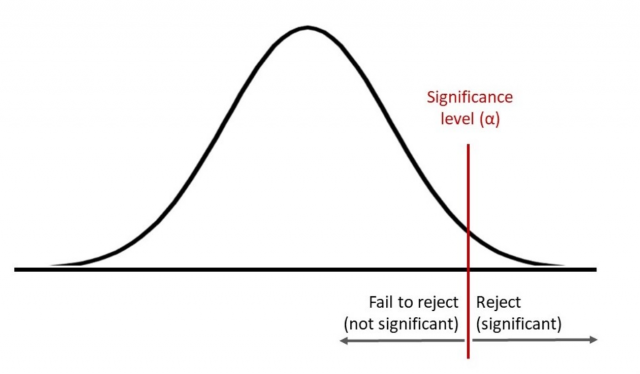
When our test statistic falls in the rejection region:
- \(p\)-value \(\leq \alpha\), thus \(H_0\) is rejected

Type II error

The probability of a Type II Error is denoted by \(\beta\)
We will talk more about this in future lectures

Type I and Type II errors

We can control the probability of type I error by our choice of the significance level, \(\alpha\)
It’s difficult to control the probability of making type II error

Take home

Hypotheses: null and alternative
Significance level: value such that we reject \(H_0\) if the \(p\)-value is less than or equal to that number
Test statistic: function of the data on which the decision based
Distribution of test statistic under null: using bootstrap or permutation
\(p\)-value: probability of observing a result as extreme or more extreme than what we observed under \(H_0\)
Draw a conclusion: reject or fail to reject \(H_0\)

\(p\)-value with simulations

\(p\)-value: probability of observing a result as extreme or more extreme towards the alternative hypothesis than what we observed given that \(H_0\) is true
- depends on \(H_A\)
- proportion of simulations that yield a sample statistic at least as favorable to the alternative hypothesis as the observed sample statistic

Today’s worksheet

Perform a range of hypothesis tests using simulations (bootstrap and permutation)

Now it’s your turn!

navigate to Canvas, open worksheet_06

We are here to help!